Anomaly Detection Using Auto Encoder

Unsupervised Way: Anomaly Detection Using Auto Encoder

Auto Encoder: Auto Encoder (AE) is an identity function where input and output are same. It is considered as an unsupervised or self-supervised learner. To build an Auto Encoder, we need three stages:

An encoding method
Decoding method
A loss function to calculate the distance between input and output.

In encoding layer, we take the input and compress the feature to lower dimension and then in decoding layer we reconstruct the input based on compressed features. Therefore, auto encoder is like Principal Component Analysis(PCA), is also considers as dimensionality reduction algorithm. One thing to note here is that Auto Encoders are built by Neural Network Architectures. The general structure of auto encoder is given as in Fig-5.

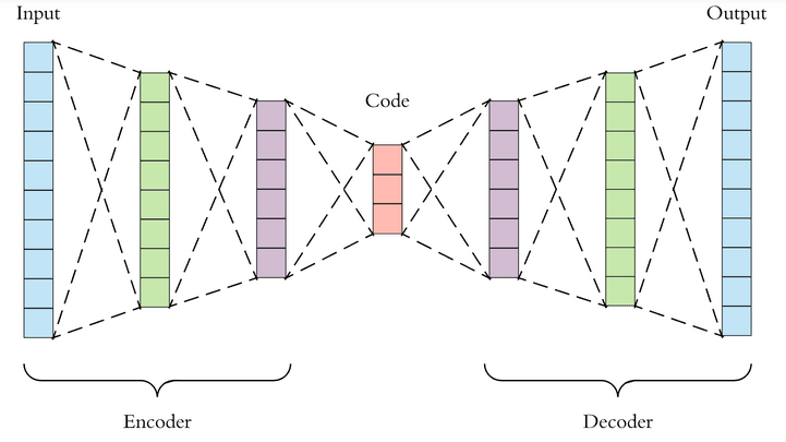
Fig -5 The general structure of an auto encoder

Source: https://towardsdatascience.com/applied-deep-learning-part-3-autoencoders-1c083af4d798

As you can see here we are taking the input with high features in the input layer, then we start compressing the dimension by reducing the neurons in the hidden layers and at the middle we get the encoded information. Now the same architecture is unrolled in the decoder side by increasing the number of neurons on subsequent hidden layers.

Anomalies are rare occurrences hence it is very difficult to obtain the data for training of models. Furthermore, anomalous behavior changes over time. Hence it becomes a necessity to classify the anomalous data at run time. Anomalies are rare occurrences hence it is very difficult to obtain the data for training of models. Furthermore, anomalous

behavior changes over time. Hence it becomes a necessity to classify the anomalous data at run time. Here our approach is to first train an auto encoder only on normal data. Then we will test the model on both normal and anomalous data. For the anomalous data, the Root Mean Square Error (RMSE) of the reconstructed data would be large.

Results and Discussion: ROC curves are a very useful tool for understanding the performance of classifiers. However, our case is a bit out of the ordinary. We have a very imbalanced dataset. Nonetheless, let’s have a look at our ROC curve:

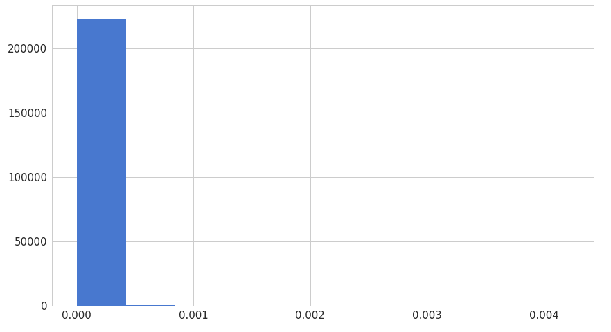
6(a). Error distribution of normal data

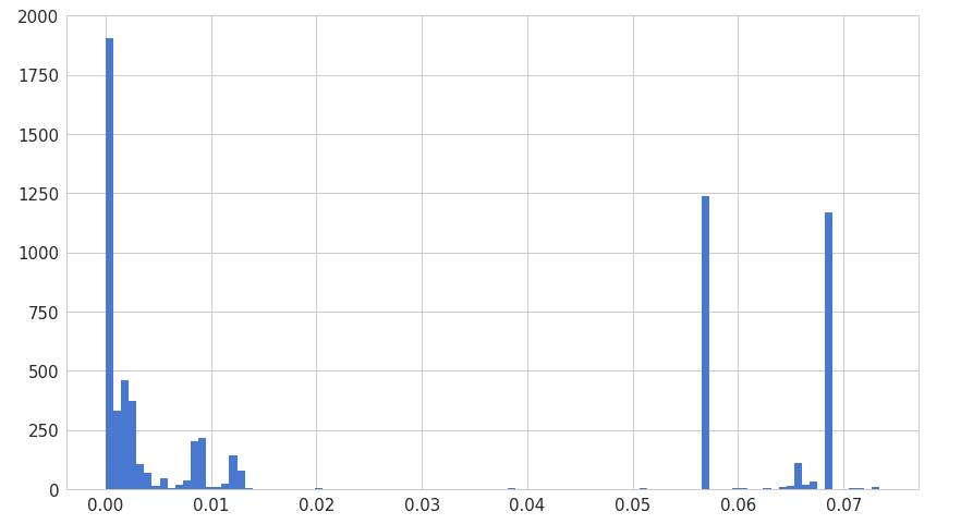
6(b). Error distribution of anomaly data

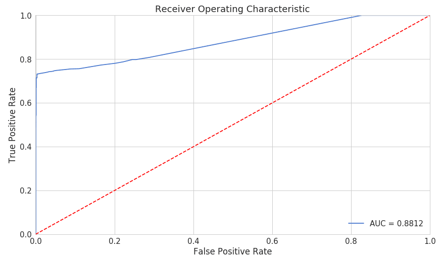
Fig -6: Error distribution of normal and anomaly data

Fig -7: Evaluation of the model based on AUC

The ROC curve plot is the true positive rate versus the false positive rate, over different threshold values. Basically, in Fig-7, we want the blue line to be as close as possible to the upper left corner. While our results look quite good, also area under the curve (AUC) value is quite high (0.88).

For AUC, the higher the value the better the model is (So more it is closer to 1 better the model). Now since our Model is trained, we have to predict whether or not a new or unseen sequence of log messages in a different time intervals or different blocks are normal or anomaly.

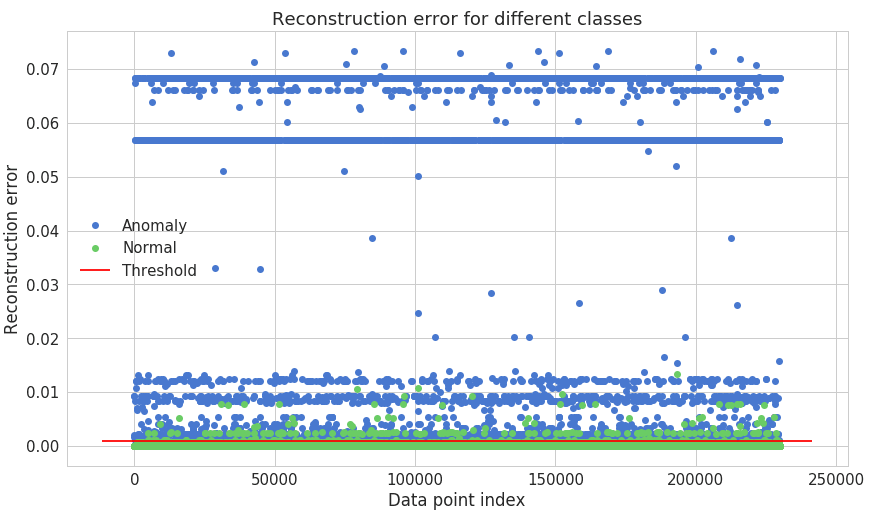
We will calculate the reconstruction error from the test data itself. If the error is larger than a predefined threshold, we will mark it as an anomaly, since our model should have a low error on normal data. In Fig-5b we make a histogram plot of error distribution of normal as well as anomaly data. By seeing the plot, we have fixed a threshold value as 0.001. Now one can observe how well the red line divide the two types of data in Fig -8:

Fig – 8 Reconstruction error for the different classes

Fig -9: Confusion matrix

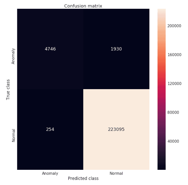
From confusion matrix in Fig-9, we have observed that our model seems to catch lot of anomalies. We have calculated precision, recall and F1 measure and the corresponding values are 0.94, 0.71, and 0.81. We can increase recall value by setting the threshold value lower than the previous one, which will decrease the fraction of anomalies misclassified as normal.